21 Lotka-Volterra competition

The Lotka-Volterra competition model is a foundational tool in ecology for understanding interspecific competition, or competition between different species for shared resources such as food, space, and nesting sites. It examines how population sizes change in a shared environment by considering factors like interaction strength and environmental carrying capacities.

The model is closely linked to the idea of “competitive exclusion”: two species with identical ecological roles cannot coexist indefinitely, and eventually one will exclude the other. This principle comes mainly from experiments, especially Gause’s work with yeasts and Paramecium in the 1930s, rather than from the model itself. In the basic model, two truly identical species do not exclude each other at all (see the fifth case below).

The model also explores the role of both inter- and intra-specific competition. It identifies conditions for species coexistence, influenced by parameters like competition coefficients and carrying capacities. These insights are vital for understanding community structure, species interactions, and ecological stability.

In a two-species system there are four general outcomes:

Predictable Exclusion of Species 1 by Species 2: Species 2 outcompetes and excludes species 1 from the environment.
Predictable Exclusion of Species 2 by Species 1: Species 1 outcompetes and excludes species 2 from the environment.
Exclusion Dependent on Initial Densities: Depending on the starting numbers of each species, either one could exclude the other.
Stable Coexistence: Both species may reach a stable equilibrium where they coexist without one excluding the other.

Neal also describes a fifth, knife-edge case, in which the two isoclines lie exactly on top of each other (see below).

The model suggests that stable coexistence is possible if each species limits its own population growth more than it affects the other species. Overlapping niches could lead to competitive exclusion, influenced by their competition coefficients and carrying capacities.

Learning outcomes:

Competence in constructing an Excel-based population model.
Understanding how the Lotka-Volterra competition model works.
Understanding the competition coefficients $\alpha$ and $\beta$, and using the isocline intercepts ($K_1$, $K_1/\alpha$, $K_2$, $K_2/\beta$) to predict the outcome of competition.

21.1 Background: the model and its isoclines

We use the notation of Neal (Interspecific Competition). Each species grows logistically, but its growth is also slowed by the other species:

\[\frac{dN_1}{dt} = r_1 N_1 \frac{K_1 - N_1 - \alpha N_2}{K_1}\]

\[\frac{dN_2}{dt} = r_2 N_2 \frac{K_2 - N_2 - \beta N_1}{K_2}\]

$\alpha$ is the per capita effect of species 2 on species 1, measured relative to the effect of species 1 on itself. If $\alpha = 0.5$, two individuals of species 2 have the same effect on species 1 as one individual of species 1.
$\beta$ is the per capita effect of species 1 on species 2, measured in the same way.

Species 1 stops growing when $N_1 = K_1 - \alpha N_2$. This straight line is the zero isocline (zero net growth isocline) of species 1. On a graph with $N_1$ on the x-axis and $N_2$ on the y-axis it crosses the x-axis at $K_1$ (no species 2 present) and the y-axis at $K_1/\alpha$ (so many individuals of species 2 that species 1 cannot grow at all). In the same way, the isocline of species 2, $N_2 = K_2 - \beta N_1$, crosses the y-axis at $K_2$ and the x-axis at $K_2/\beta$. Each species increases when the populations are below (to the left of) its own isocline and decreases above it.

The outcome depends on how the two isoclines are arranged (Fig. 21.1):

Arrangement of the intercepts	Outcome
$K_1 > K_2/\beta$ and $K_1/\alpha > K_2$ (species 1’s isocline lies outside species 2’s)	Species 1 excludes species 2
$K_2 > K_1/\alpha$ and $K_2/\beta > K_1$ (species 2’s isocline lies outside species 1’s)	Species 2 excludes species 1
$K_1 < K_2/\beta$ and $K_2 < K_1/\alpha$ (the isoclines cross)	Stable coexistence at the crossing point
$K_1 > K_2/\beta$ and $K_2 > K_1/\alpha$ (the isoclines cross the other way)	Unstable equilibrium: either species can win, depending on the starting densities

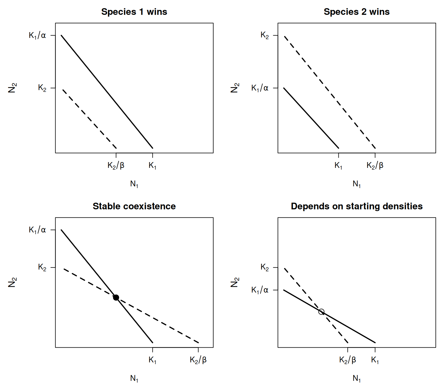
$The four general arrangements of the Lotka-Volterra competition isoclines. Solid line: species 1 (intercepts $K_1$ and $K_1/\alpha$). Dashed line: species 2 (intercepts $K_2$ and $K_2/\beta$). Filled circle: stable equilibrium; open circle: unstable equilibrium.$

Figure 21.1: The four general arrangements of the Lotka-Volterra competition isoclines. Solid line: species 1 (intercepts $K_1$ and $K_1/\alpha$). Dashed line: species 2 (intercepts $K_2$ and $K_2/\beta$). Filled circle: stable equilibrium; open circle: unstable equilibrium.

In the fifth case (Neal’s “coexistence at a range of equilibrium densities”), $K_1 = K_2/\beta$ and $K_2 = K_1/\alpha$, so the two isoclines lie exactly on top of each other. Every point on the shared line is an equilibrium, and the species coexist at whatever ratio they happen to reach. Two identical species ($\alpha = \beta = 1$, $K_1 = K_2$) are an example. This case needs exactly matching values, so it is unlikely in nature. It also shows that the basic model does not, on its own, predict the exclusion of identical species: Gause observed exclusion in his Paramecium experiments, and Neal shows that an extra source of mortality (a “removal factor”) has to be added to the model to explain it.

21.2 Key idea

Whether a coefficient is bigger or smaller than 1 does not decide the outcome on its own. What matters is how each competition coefficient compares with the ratio of the carrying capacities. The easiest way to see this is to ask whether each species can invade when it is rare and the other species is sitting at its carrying capacity.

Species 1 can invade a population of species 2 at $K_2$ if $K_1 > \alpha K_2$, i.e. if $\alpha < K_1/K_2$ (equivalently $K_2 < K_1/\alpha$).
Species 2 can invade a population of species 1 at $K_1$ if $K_2 > \beta K_1$, i.e. if $\beta < K_2/K_1$ (equivalently $K_1 < K_2/\beta$).

Species 1 can invade?	Species 2 can invade?	Outcome
Yes	No	Species 1 excludes species 2
No	Yes	Species 2 excludes species 1
Yes	Yes	Stable coexistence
No	No	Exclusion, but which species wins depends on the starting densities

These are the same conditions as in the isocline table above, written in a different way.

For example, with $K_1 = 3000$, $\alpha = 1.25$, $K_2 = 1000$ and $\beta = 0.5$, species 2 has the stronger per capita effect ($\alpha > 1$), yet species 1 wins: species 1 can invade ($1.25 < 3000/1000 = 3$) but species 2 cannot ($0.5 > 1000/3000 = 0.33$).

21.3 Your task

In this class (over TWO sessions) you will be working from a PDF available here to make a model exploring this idea.

This PDF walks you through the creation of an Excel spreadsheet exploring interspecific competition and competitive exclusion using the Lotka-Volterra model.

Notation and time steps in the PDF

The PDF writes the competition coefficients as $\alpha_{12}$ and $\alpha_{21}$. In Neal’s notation (used in this book), $\alpha_{12} = \alpha$ (effect of species 2 on species 1) and $\alpha_{21} = \beta$ (effect of species 1 on species 2).
The spreadsheet is a discrete-time version of the model: $N_{1,t+1} = N_{1,t} + R_1 N_{1,t}(K_1 - N_{1,t} - \alpha N_{2,t})/K_1$, and the same for species 2. Its $R$ is a rate per time step, not Neal’s continuous $r$. Keep $R_1$ and $R_2$ at 1 or below, so that you see the Lotka-Volterra behaviour rather than the oscillations and chaos of the discrete logistic model (compare Deeper into logistic growth).

Create the Excel spreadsheet by following the instructions in the PDF.

Note on the PDF: the labels added to Figure 5 have the subscripts the wrong way round. The correct isocline intercepts are $K_1$ and $K_1/\alpha_{12}$ for species 1, and $K_2$ and $K_2/\alpha_{21}$ for species 2 (in Neal’s notation, $K_1$, $K_1/\alpha$, $K_2$ and $K_2/\beta$; see the Background above).

In the first session, build the sheet and check it: with the PDF’s default values ($R_1 = R_2 = 1$, $K_1 = 1200$, $\alpha = 0.75$, $K_2 = 1000$, $\beta = 0.5$, starting at $N_1 = 100$, $N_2 = 50$) the two species should settle at $N_1 = 720$, $N_2 = 640$. Label the four isocline intercepts on your graph.
In the second session, use the model to answer the questions below. For each parameter set you try, sketch the isoclines and predict the outcome first, then run the model to check.

21.3.1 The questions

What parameter values will cause species 1 to exclude species 2 from the habitat? What do these values mean in ecological terms?
What parameter values will reverse this outcome? What do these values mean in ecological terms?
What parameter values will allow the two species to coexist indefinitely and stably? What do these values mean in ecological terms?
Are there parameter values under which the outcome depends on initial population sizes or rates of population growth? What do these values mean in ecological terms?
(Optional) Neal describes two pairs of flour beetles. Predict the outcome for each from the isoclines, then check with your sheet: (a) Rhizopertha (species 1, $K_1 = 330$) and Oryzaephilus (species 2, $K_2 = 440$), with $\alpha = 0.235$ and $\beta = 0.12$; (b) Tribolium confusum (species 1, $K_1 = 220$) and T. castaneum (species 2, $K_2 = 340$), with $\alpha = 1$ and $\beta = 2.2$. For (b), try several different starting densities.

21.4 Takeaways

Competition outcomes depend on relative self-limitation vs. interspecific effects.
The competition coefficients $\alpha$ and $\beta$ encode how much one species suppresses the other.
Coexistence occurs when each species limits itself more than it limits the other, in the scaled sense that $\alpha < K_1/K_2$ and $\beta < K_2/K_1$ (each species can invade when rare). Comparing a coefficient with 1 is not enough when the carrying capacities differ.
The four isocline intercepts ($K_1$, $K_1/\alpha$, $K_2$, $K_2/\beta$) are all you need to predict the outcome.

Arrangement of the intercepts	Outcome
\(K_1 > K_2/\beta\) and \(K_1/\alpha > K_2\) (species 1’s isocline lies outside species 2’s)	Species 1 excludes species 2
\(K_2 > K_1/\alpha\) and \(K_2/\beta > K_1\) (species 2’s isocline lies outside species 1’s)	Species 2 excludes species 1
\(K_1 < K_2/\beta\) and \(K_2 < K_1/\alpha\) (the isoclines cross)	Stable coexistence at the crossing point
\(K_1 > K_2/\beta\) and \(K_2 > K_1/\alpha\) (the isoclines cross the other way)	Unstable equilibrium: either species can win, depending on the starting densities