31 Continuous traits from discrete genes
31.1 Background
This activity uses a fast classroom simulation to show how many small genetic effects can generate a continuous, approximately normal trait distribution. It connects to the heritability workflow in 3_04_Heritability.Rmd.
Learning outcomes:
- Explain how additive genetic effects create continuous trait variation.
- Compare a classroom simulation with a simple R simulation.
31.2 Worked example
31.3 Your task
Use the intuition exercise in supplemental/Quantitative_Genetics/Continuous_Traits_From_Discrete_Genes.docx and the spreadsheet in supplemental/Quantitative_Genetics/Continuous_Traits_From_Discrete_Genes.xlsx.
- In class, treat each student as a gene that can be ON (1) or OFF (0). Choose a baseline trait value of 35, and add 1 for each ON gene. Record the trait value for at least 30 individuals.
- Plot a quick histogram of the observed trait values. Describe the shape.
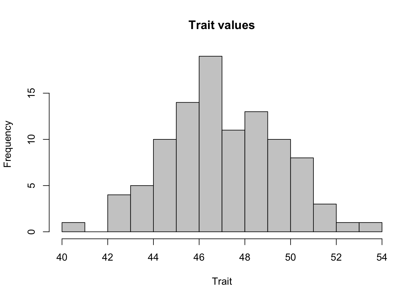
- Now simulate the same process in R for 100 individuals and 25 genes. Compare your histogram to the classroom version.
- Relate the outcome to the concept of additive genetic variance in
3_04_Heritability.Rmd.
set.seed(123)
baseline <- 35
n_genes <- 25
n_individuals <- 100

gene_on <- rbinom(n_individuals, size = n_genes, prob = 0.5)
trait_value <- baseline + gene_on

hist(trait_value, breaks = 12, col = "gray80", main = "Trait values", xlab = "Trait")