27 Exponential growth in detail
One of the foundational concepts in population dynamics is the exponential growth model. This model is a simplified representation of how populations grow when resources are not limiting. While it’s rare for populations to experience uninhibited growth for extended periods, understanding this basic model is crucial for understanding more complex dynamics that include factors like resource limitations, predation, and disease.
In this chapter, we will explore the mathematical framework that describes exponential growth in both discrete and continuous time settings. We will introduce key parameters such as the per-capita birth rate, death rate, and intrinsic rate of increase. We will also demonstrate how to apply these models using R programming, offering a practical dimension to these theoretical concepts.
Learning outcomes:
- Understand the fundamental equations that underpin exponential growth in populations.
- Differentiate between discrete and continuous time models.
- Interpret the role and significance of various parameters in exponential growth models.
- Use R programming to analyse exponential growth scenarios with real data.
27.0.1 Nomenclature
| Symbol | Meaning | Alternatives |
|---|---|---|
| \(R\) | Per capita rate of increase, per capita population growth rate | \(R_m\) (Neal), \(r\) (Gotelli), \(r_c\) is used as the \(R\) estimated from a life table in Neal |
| \(r\) | Intrinsic rate of increase | \(r_m\) |
| \(\lambda\) | Population growth rate, population multiplication rate | |
| \(R0\) |
27.1 Discrete time model
We’ll first look at discrete population growth, which is the population growth that is considered to grow over distinct time steps (e.g., 1 year intervals). This is also called Geometric Population Growth.
A population at time \(t\) has size \(N\): \(N_t\).
After one time interval, there will be some births (\(B\)), and some deaths (\(D\)). Births will have the effect of increasing the population size at time \(t+1\) while deaths will decrease population size. The population at the next time step (\(N_{t+1}\)) is thus:
eqn. 1. \(N_{t+1} = N_t + B - D\)
We can think about the birth/death processes on a per-individual basis, and use per-capita birth rate (\(b\)) and per-capita death rate (\(d\)). We can think of \(b\) as the average number of offspring produced by an individual during the time interval starting at \(N_t\) and ending at \(N_{t+1}\). Similarly, \(d\) is the probability that an individual alive at \(N_t\) will die at some point during the interval.
The total number of births within a time interval depends on the number of individuals there are at the start of the interval (\(N_t\)), and the total number of births in the population during the time interval is \(bN_t\). Similarly, the total number of deaths is \(dN_t\). Thus:
eqn. 2. \(N_{t+1} = N_t + bN_t - dN_t\).
This equation can be simplified to:
eqn. 3. \(N_{t+1} = N_t + (b-d)N_t\).
Furthermore, because the expression \((b-d)\) is important, we can give it its own symbol, \(R\). \(R\) is called the per capita rate of increase or the intrinsic rate of increase. (Note that the nomenclature varies depending on the book/paper! In other places this is called \(r_d\), or \(R_m\)).
So we now have:
eqn. 4. \(N_{t+1} = N_t + RN_t\).
Or, if we are only interested in the change in population size:
eqn. 5. \(\frac{\Delta N}{\Delta t} = RN_t\).
Equation 4 can be simplified again, by factoring out the \(N_t\) on the right hand side:
eqn. 6. \(N_{t+1} = (R + 1)N_t\).
The quantity \((R+1)\) is given its own symbol: \(\lambda\), the population multiplication rate (also known as the “finite rate of increase”).
eqn. 7. \(N_{t+1} = \lambda N_t\).
By rearranging this equation (eqn. 7) we can see that \(\lambda\) is simply the ratio of population size at time \(t+1\) and \(t\):
eqn. 8. \(\lambda = N_{t+1}/N_t\).
It follows, therefore, that when the population is neither growing nor declining (when \(N_{t+1}=N_t\)), \(\lambda = 1\) (and when \(R\) = 0).
27.1.1 Calculating N for any future time point
Assuming the population growth rate remains constant, we can calculate the population at any time in the future.
As a starting point, consider equation 7: \(N_{t+1} = \lambda N_t\).
If we want to calculate \(N_{t+2}\), we would need to plug in \(N_{t+1}\) instead of \(N_t\): \(N_{t+2} = \lambda N_{t+1}\),
and, since we know that \(N_{t+1} = \lambda N_t\),: \(N_{t+2} = \lambda \lambda N_t\).
Similarly, if we wanted to calculate \(N_{t+2}\), we’d end up with: \(N_{t+3} = \lambda \lambda \lambda N_t\).
This can be simplified by raising \(\lambda\) to a suitable power, and using the starting population at time = 0, \(N_0\):
eqn. 9. \(N_{t} = \lambda ^tN_0\).
This should be familiar to those of you that did (or remember!) the concept of geometric series which was covered in MM554 Mathematics for Biology.
27.1.2 Applying the model
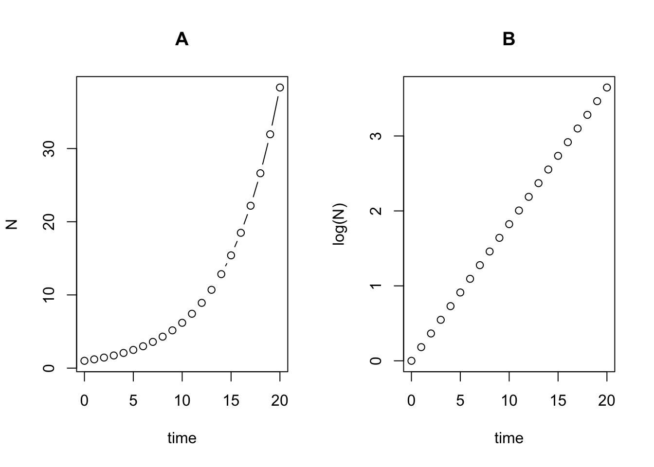
If we plot exponential growth on a log scale we can see that it is straight line. For example, in the plot below I show the sequence for a population with a starting population of 1 and a \(\lambda\) (population multiplication rate) of 1.2 (i.e., the population increases by 20% each year). In (A) the time series is plotted on the natural scale while in (B) it is plotted on the log scale.
# Load required libraries
require(tidyverse)

# Set initial population and lambda
startPop <- 1
lambda <- 1.2

# Create a data frame with time and corresponding population
df1 <- data.frame(time = 0:20) %>%
  mutate(N = lambda^time * startPop)
# Plotting the data
par(mfrow=c(1,2))
# Plot on natural scale
plot(df1$time, df1$N, type = "b", xlab = "time", ylab = "N")
title("A")
# Plot on log scale
plot(df1$time, log(df1$N), type = "b", xlab = "time", ylab = "log(N)")
title("B")
In fact, we can linearise the relationship by log transforming both sides of equation 9:
\(\ln{N_t} = \ln(\lambda ^tN_0)\),
which can be re-written as:
\(\ln{N_t} = \ln(\lambda )t + \ln(N_0)\).
This looks familiar. Indeed, the equation of a straight line (\(y = ax + b\)) maps onto this. In this equation, the slope \(a\) is equivalent to \(\ln(\lambda )\) and the intercept (\(b\)) is equivalent to \(\ln(N_0)\).
This is very convenient because now we can use simple regression methods to estimate \(\ln(\lambda)\) (the slope) of the relationship, and therefore the value of \(\lambda\) (or \(R\), which is \(\lambda -1\)).
27.2 Real-World Application: Breeding Pairs of Merlin (Falco columbarius)
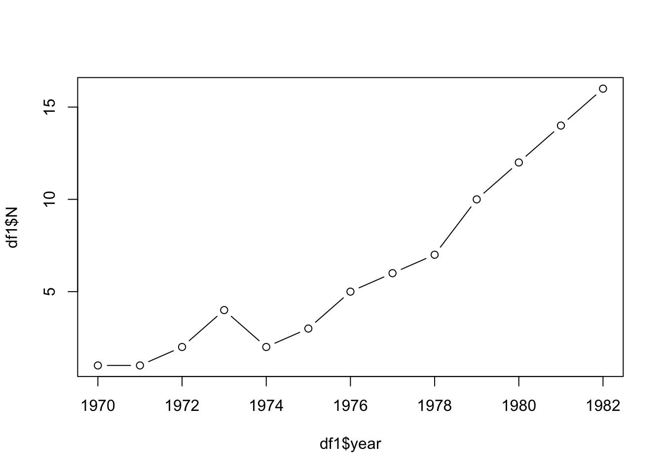
To bring these mathematical concepts to life, let’s consider an example from the Neal textbook that focuses on the population of breeding pairs of Merlin, a species of small falcon. The data spans from 1970 to 1982 and shows the following population sizes (breeding pairs): 1,1,2,4,2,3,5,6,7,10,12,14,16
This is not much data, so we can simply put it into R manually, and plot it, like this:
df1 <- data.frame(year = 1970:1982,
                  N = c(1,1,2,4,2,3,5,6,7,10,12,14,16))
plot(df1$year,df1$N, type = "b")
27.2.1 Observations and Context
It is clear from the graph that the number of breeding pairs is increasing over the years, albeit with some fluctuations. These fluctuations could be due to various factors such as changes in food availability, predation, or human activity. However, the general trend suggests growth.
27.2.2 Applying the Exponential Growth Model
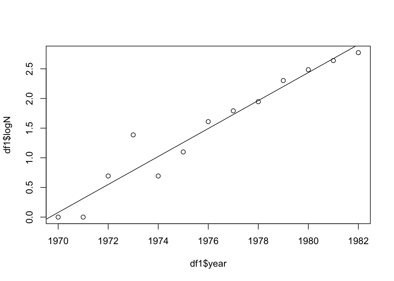
To analyse this data, we’ll use the exponential growth model. We’ll plot the data on a log scale and fit a regression model:

Model summary output:
##
## Call:
## lm(formula = logN ~ year, data = df1)
##
## Residuals:
##      Min       1Q   Median       3Q      Max
## -0.32858 -0.13684 -0.01967  0.10104  0.60054
##
## Coefficients:
##               Estimate Std. Error t value Pr(>|t|)
## (Intercept) -464.77072   36.12270  -12.87 5.66e-08 ***
## year           0.23596    0.01828   12.91 5.48e-08 ***
## ---
## Signif. codes:  0 '***' 0.001 '**' 0.01 '*' 0.05 '.' 0.1 ' ' 1
##
## Residual standard error: 0.2466 on 11 degrees of freedom
## Multiple R-squared:  0.9381, Adjusted R-squared:  0.9324
## F-statistic: 166.6 on 1 and 11 DF,  p-value: 5.478e-08
Interpretation
The summary of the model indicates that the slope of the relationship between year and logN is 0.2359637. Therefore, the per capita growth rate (\(R\)) is 0.236 and the population multiplication rate (\(\lambda\)) is 1.236.
This suggests that the number of breeding pairs is indeed growing exponentially over the time period studied, with a specific rate of increase. Understanding this rate is crucial for conservation efforts, because it provides insights into the population’s resilience, its demands on the ecosystem, and how it might respond to future changes in environmental conditions or conservation policies.
27.3 Continuous time model
In contrast to the discrete time model, the continuous time model allows us to understand population growth without the constraint of clear time intervals. This is particularly useful for studying populations that don’t have breeding seasons or for those that experience continuous births and deaths (e.g. bacteria, humans).
The starting point for the continuous time model is the intrinsic rate of increase, \(r\). This is defined as: \(r = ln(\lambda)\) which is the same as saying \(r = ln(N_{t+1}/N_t)\)
We say that \(r = ln(\lambda)\) “r is the natural log of lambda”.
Here, \(\lambda\) is the population multiplication rate, as discussed in the discrete time model section. The natural logarithm of \(\lambda\) gives us \(r\), which can be interpreted as the rate of population growth per unit time when resources are unlimited.
To back-transform from a natural log, we use the exponential. Therefore, \(\lambda = e^r\): “lambda is the exponential of r”.
This allows us to relate \(\lambda\) and \(r\) directly. From the discrete model (above), we know that \(\lambda = 1 + R\), so:
\(1+R = e^r\)
\(R = e^r - 1\)
27.3.1 Zero population growth
When the population is steady with zero growth, \(r = 0\) and \(\lambda = 1\). It’s important to note that the relationship \(\lambda = r + 1\) only holds true when the population is not growing or shrinking. This is a special case and should not be generalised. Do not make the common mistake to think that \(\lambda\) is simply \(r + 1\)!