13 Life Table Response Experiments

13.1 Introduction

A Life Table Response Experiment (LTRE), in matrix population modelling, is a technique used to analyse how differences in demographic parameters between two or more populations or “treatments” contribute to differences in their overall growth rate. It’s particularly useful for understanding how specific factors like survival rates, fecundity, or other stage-to-stage transitions influence the growth or decline of a population under different conditions.

The method involves comparing matrix models of the populations in question and decomposing the differences in growth rates different models into contributions from individual matrix elements. This approach provides insights into which life cycle stages or transitions are most important for population growth and can inform conservation or management strategies.

13.2 Set up

First we need to ensure that we have the R packages we need loaded. If you get an error doing this, remember to install them first (install.packages("PACKAGE_NAME"))

library(popbio)
library(popdemo)
library(Rcompadre)

13.3 A worked example

In this example, we consider a two-stage matrix model to analyze, say, squirrel populations in two different geographic locations. The first, a reference population from Location A, represents an area with favorable environmental conditions. The matrix model for this population distinguishes between juveniles (J) and adults (A), incorporating probabilities for juveniles maturing into adults (0.5) and adults surviving and staying adult (0.6), as well as the fecundity rate (2.3), which is the number of juveniles produced by an adult.

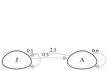
The treatment population, from Location B, experiences generally worse environmental conditions during the spring which particularly impacts the juvenile stages, and includes an effect on fecundity (e.g. via neonatal maternal energy allocation). The two matrices can be created in R as follows. Compare the values in the matrix, to the values in the life cycle diagram.

A_ref <- matrix(c(0.1,2.3,
                  0.5,0.6), nrow = 2, ncol = 2, byrow = TRUE)

A_treat <- matrix(c(0.1,1.3,
                    0.2,0.7), nrow = 2, ncol = 2, byrow = TRUE)

13.3.1 Comparing matrices

Before we dig into the formal LTRE, it is useful to compare the two matrices, A_ref and A_treat, to see how they are different from eachother.

We can check what overall difference there is between the matrix in a couple of ways.

Firstly, we can examine the differences in the individual transition rates between the matrices by subtracting one from the other.

A_ref - A_treat

##      [,1] [,2]
## [1,]  0.0  1.0
## [2,]  0.3 -0.1

Next, we can ask what impact these differences have on the population growth rate (lambda). Note that putting the command in parentheses tells R to both create the new object (e.g. lambdaA1) and print the result to the screen.

(lambda_A_ref <- eigs(A_ref, what = "lambda"))

## [1] 1.451136

(lambda_A_treat <-eigs(A_treat, what = "lambda"))

## [1] 0.991608

We could express this as a difference, or as a proportional difference.

The difference in growth rates between the matrices is 0.46.

(lambdaDiff <- lambda_A_ref - lambda_A_treat)

## [1] 0.4595278

This is a 32% reduction, compared to the reference matrix.

(lambdaDiff/lambda_A_ref) * 100

## [1] 31.66677

So far, so good. We can see that treatment reduces the population growth rate, but we don’t know exactly how. There are 3 changes in the matrix. Which of these changes is most instrumental in driving change in the population growth rate?

13.3.2 Contributions from individual matrix elements

The objective of the LTRE (Life Table Response Experiment) analysis in this context is to understand the impact of these environmental differences on the difference in population growth rate between the two populations. This is important because identifying the specific life history traits (i.e. the individual transitions, represented by individual elements of the matrix, such as survival or fecundity) that are most sensitive to environmental changes allows us to pinpoint the key drivers of population dynamics.

By understanding where differences in growth rate originate, we can make more informed decisions about conservation and management strategies. For instance, if the analysis shows that adult survival has a larger impact on growth rate than fecundity, conservation efforts can be more effectively focused on improving adult survival rates rather than fecundity. Conversely, if juvenile survival or fecundity is more influential, efforts might be better directed towards enhancing these aspects. This targeted approach ensures that resources are allocated efficiently, and interventions are tailored to address the most critical factors affecting the population’s viability under varying environmental conditions.

By comparing the two models, we can decompose the differences in the overall growth rate (\(\lambda\)) between the baseline (Location A) and the modified model (Location B). This analysis will specifically highlight how changes in adult survival and fecundity in the less favorable environment of Location B contribute to any differences in population growth rates compared to the more favorable conditions in Location A. Such insights are crucial for developing effective management and conservation strategies, particularly in understanding the relative importance of different life stages and demographic parameters under varying environmental conditions.

popbio::LTRE(A_treat,A_ref)

##            [,1]        [,2]
## [1,]  0.0000000 -0.20832964
## [2,] -0.3214229  0.06636876

This summary quantifies the relative importance (and direction) of the effect of the differences between the two matrices on the difference in population growth rate. One of the changes actually has a positive impact on growth rate, but this is opposed by the other two changes. The most important of these two is the lower left element, which represents the ontogenetic development from juvenile to adult stage.

13.4 Relationship with elasticity analysis

There are similarities between LTRE analysis and elasticity analysis. Comparing LTRE with elasticity analysis reveals some distinct advantages of LTRE in certain contexts.

LTRE can handle comparisons where changes occur in multiple life history parameters simultaneously, providing a more comprehensive view of the potential impacts of various factors on population dynamics. This is in contrast to elasticity analysis, which examines the sensitivity of the population growth rate to small changes in individual demographic rates and assumes other parameters remain constant.

Therefore, LTRE is more directly applicable for evaluating and comparing the impacts of different management strategies or environmental changes that simultaneously affect several demographic traits. It allows for a more nuanced understanding of how specific interventions (like changes in fecundity or survival rates) will influence the population. This is crucial for making informed decisions in conservation and wildlife management.

In summary, while elasticity analysis is valuable for understanding the inherent sensitivity of a population’s growth rate to changes in its life cycle processes, LTRE can be a more useful tool for analyzing the more complex effects of environmental variations or different management strategies on population dynamics.