6 Stochastic population growth
6.1 Background
In contrast to the deterministic nature of the geometric growth model, a stochastic version of the model introduces an element of randomness, making it more reflective of real-world scenarios. Instead of assuming fixed and predictable growth rates, the stochastic model incorporates uncertainties and fluctuations that occur due to various factors, such as environmental variability, chance events, and individual-level variations in reproductive success. By embracing this stochastic approach, the population dynamics become more realistic, allowing us to better understand and predict the inherent variability and uncertainties associated with natural populations. This stochastic framework provides a valuable tool for ecologists and researchers to explore the dynamics of real populations under more complex and dynamic conditions.
Remember – this model still allows for unbounded population growth – the populations are not influenced by population density.
We’ll focus on the discrete (Geometric) growth model: \(N_{t+1}=\lambda N_t\).
Because \(\lambda = \mathrm{e}^{r_m}\) (and \(r_m = ln(\lambda)\)), we can rearrange the equation to express it as \(N_{t+1}=\mathrm{e}^{r_m} N_t\).
Therefore, we can predict next year’s population size from this year’s population if we know either \(r_m\) or \(\lambda\).
We will create some models in Excel, and then in R, to explore the effect of stochastic variation in the population growth rate.
We can simulate variation in \(r_m\) by drawing a random number from a normal distribution with a particular mean (\(\bar{r_m}\)) and variance (\(\sigma_{r_m}^2\)) (Fig. 6.1). The \(\bar{r_m}\) value determines the long-term average while the \(\sigma_{r_m}^2\) estimates how much “spread” there is in the data from year to year.
In the figure you can see that the peak of the \(r_m\) distribution is \(>0\) (approximately 0.1), so on average, the population will tend to grow. However, in poor years \(r_m\) is \(<\) 0, so the population will decline in those cases. Both the mean value and the spread of the distribution (i.e. variance) determine the fate of the population.
Remember that we can convert \(r_m\) to \(\lambda\) by taking the exponential, because \(r_m = ln(\lambda)\).
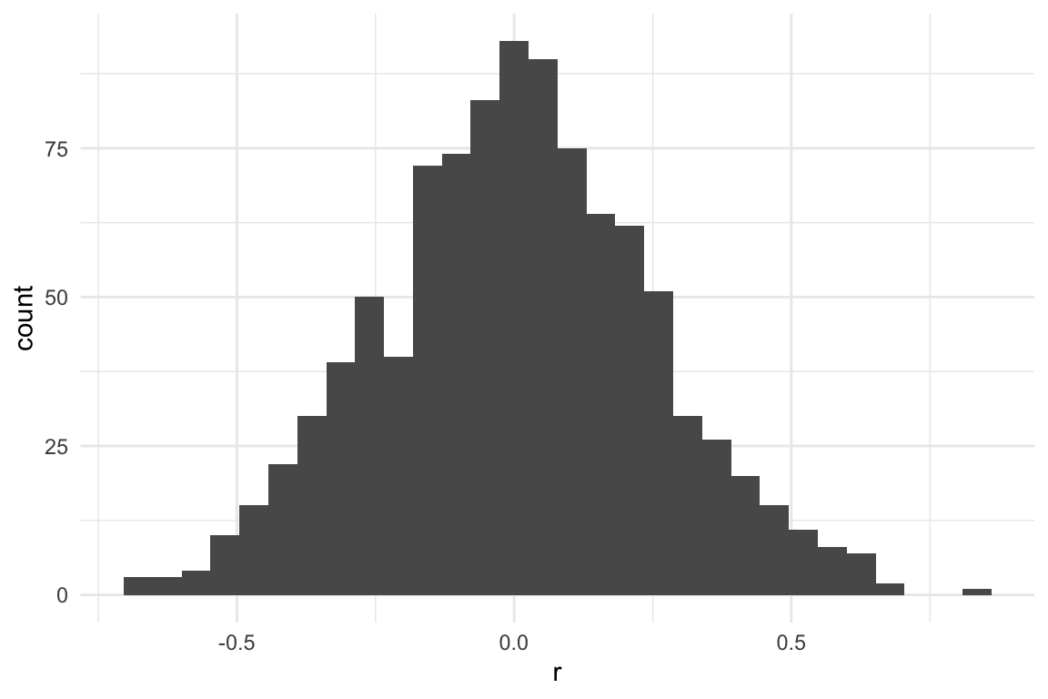
Figure 6.1: A normal distribution of potential r values
When using the equation above to calculate population at time \(t+1\) (\(N_{t+1}\)) from the population at time \(t\) (\(N_t\)), one would draw a random \(r_m\) value from this distribution. Sometimes \(r_m\) will be high, other times it will be low, most of the time it will be from around the middle of the distribution.
Learning outcomes:
- Increased competence in using Excel formulae for mathematical modeling.
- Understanding the concept of stochasticity in simple population models.
- Competence in using mathematical models in Excel to strengthen own understanding of biological processes.
- Understanding how stochasticity relates to (i) uncertainty in the prediction of population trajectories and (ii) probability of (local) extinction.
6.2 Your task
Use the Excel worksheet, StochasticPopulationGrowth.xlsx, to study how stochastic population growth works with this simple model.
If \(r_m\) is drawn from a distribution with mean 0.05 and variance 0.1, then most years are positive but some are negative. This means a population can grow on average yet still crash by chance, especially when starting size is small.
- Use Excel formulae to calculate deterministic population size through time (20 generations, with starting population of 100), linking to the mean finite population growth rate.
- Use charts to plot the results. (you already did this last time!)
- Use a formula to generate a column of stochastic \(r_m\) values, based on a chosen mean and variance. In English versions of Excel the function may be written either as
=NORM.INV(RAND(), $F$10, SQRT($F$11))(newer versions) or=NORMINV(RAND(), $F$10, SQRT($F$11))(older versions), while in Danish Excel it appears as=NORMINV(SLUMP(); $F$10; KVROD($F$11)). If you encounter errors, check whether your copy of Excel expects commas or semi-colons as argument separators and adjust the formula accordingly. - Use the same procedure as before, to create a stochastic population size vector (stochastic N). Remember to convert \(r_m\) to \(\lambda\) by taking the exponential.
- Compare the two trajectories using a chart.
- Try altering initial population size, mean population growth, and the amount of stochasticity (Variance).
- Extinction occurs when N \(\leq\) 0. What happens to extinction risk as stochasticity (variance) increases? What happens when initial N is small? Does the population ALWAYS survive if the population growth rate, \(r_m\) is \(>\) 0?
Note: Excel re-randomises the random numbers every time you change any cell in the sheet. This is OK, and allows you to explore a stochastic simulation many times.
6.3 Simulations in R
Excel is of limited use to really get a feel for this. For the next part we’ll use R.
If you already have R on your computers you can play along, otherwise take a look at my demonstration in class. I will show how you can use this simulation approach to estimate extinction risk and how this is related to starting population size, mean lambda, and the amount of stochasticity.
You can copy/paste the code below into R.
The output of the modelling is shown in Fig. 6.2
Copy-and-paste the code below into a text file (or directly into R).
The final line of the code (nExtinct/nTrials) gives you an estimate of extinction probability - the proportion of trials that lead to a population size of 1 (or less).
Modify the simulation settings to explore what happens to (i) the plot of population growth and (ii) extinction risk, when you vary mean.r (\(\bar{r_m}\)), the amount of stochasticity (\(\sigma_{r_m}^2\)) (var.r), and the number of generations (nGen).
#Simulating stochastic geometric population growth rate

#Simulation settings (try changing these)
mean.r = 0.05 # the mean value of r
var.r = 0.1 # the variance in r (stochasticity)
startPop = 10 # pop size at start
nGen = 50 # number of generations
nTrials = 100 # number of repeated simulations

##########################################################
#If you are unfamiliar with R, don't edit below this line!
##########################################################

pseudoExtinction = 1

# First randomly generate some r values
rValues <- matrix(rnorm(nTrials * nGen,
                        mean = mean.r,
                        sd = sqrt(var.r)),
                  ncol = nTrials,
                  nrow = nGen)

# Use a histogram to see what they look like
# (uncomment the line below)
# hist(rValues,col="grey",main="")

# Now run the simulations to see what the resulting
#population growth looks like
trials = matrix(data = NA, nrow = nGen, ncol = nTrials)
for (j in 1:nTrials) {
  popSize = startPop
  for (i in 2:nGen) {
    stoch.r = rValues[i, j]
    popSize = append(popSize, popSize[i - 1] * exp(stoch.r))
  }
  trials[, j] = popSize
  rm(popSize)
}

#Calculate probability of (pseudo)extinction
minvals <- apply(trials, 2, min)
nExtinct <- length(minvals[minvals <= pseudoExtinction])
probExtinct <- nExtinct / nTrials
cat("Pseudo-extinction probability:", round(probExtinct, 3), "\n")
## Pseudo-extinction probability: 0.086.3.1 Example stochastic trajectories
#Make a plot of the population trajectories
plot(
  1:nGen,
  log(seq(0.1, max(trials), length.out = nGen)),
  type = "n",
  axes = F,
  xlab = "Time",
  ylab = "log(N)",
  ylim = log(c(0.1, 100000))
)
matlines(log(trials),
         col = "#FF234520",
         lty = 1,
         lwd = 3)
axis(1)
axis(2,
     at = log(c(0.1, 1, 10, 100, 1000, 10000, 100000)),
     labels = c(0.1, 1, 10, 100, 1000, 10000, 100000))
abline(h = log(pseudoExtinction), lty = 2)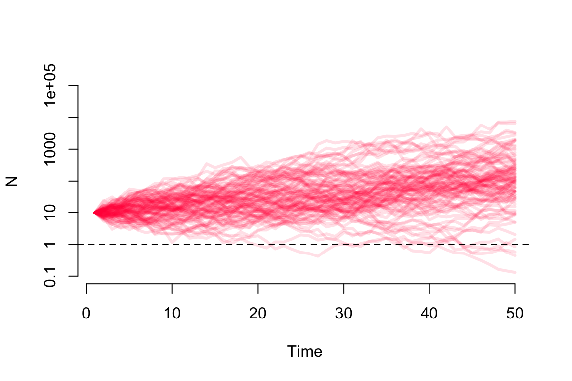
Figure 6.2: An example of stochastic population projection (100 simulations for 50 generations)
6.4 Things to try
Work through these experiments and note what happens to (a) the plot and (b) the extinction probability each time.
- Run the code as-is. Note the extinction probability and the spread of trajectories.
- Keep
mean.r = 0.05but increasevar.rto 0.5. How does extinction risk change? - Reset
var.r = 0.1, then reducestartPopfrom 10 to 3. Does starting population size matter? - Set
mean.r = 0.0(population neither growing nor shrinking on average). Is extinction certain, unlikely, or somewhere in between? - Challenge: find a combination of
mean.randvar.rwheremean.r > 0but extinction probability exceeds 0.5. What does this tell you?
6.5 Questions
- What is the main difference between deterministic and stochastic population growth models?
- Describe how incorporating randomness into the stochastic model makes it more realistic for understanding real-world populations.
- Simulate a scenario where two populations with identical growth rates experience different outcomes due to stochastic factors. Explain the implications of these findings.
- What can this stochastic model tell us about extinction risk and population size?
- What can this stochastic model tell us about extinction risk and environmental variation?
6.6 Takeaways
- Stochasticity introduces variability in trajectories.
- Even when the average growth rate is positive, stochastic variation can create a real risk of extinction.
- Small populations are more vulnerable to random declines and extinction.
- The variance of \(r\) can be as important as its mean for long-term population persistence. This is why conservationists worry about increasing environmental variability, not just declining average conditions.
- Running a model many times (as in the R simulation) reveals the distribution of possible outcomes — a much richer picture than any single trajectory provides.