17 The Gene Pool Model
17.1 Background
A central goal in evolutionary biology is to understand variation – including genetic variation – and how it changes through time. One important idea is the “gene pool,” which contains all the different versions of genes within a group of organisms. These genes/alleles determine phenotype traits and other characteristics. To grasp how populations evolve, we need to understand how allele frequencies change in a population. Over time, genetic diversity changes as the relative numbers of alleles changes. Some alleles may be lost from the population while others may become “fixed” – where the allele is present in every individual in the population.
The primary factor that influences genetic drift in the gene pool model is population size. In small populations, “sampling error” means that, just by chance, large changes often occur in the allele frequencies. In large populations, dramatic changes are much less likely.
Two related concepts are critical in understanding genetic drift: bottlenecks and founding effects. A genetic bottleneck occurs when a population dramatically reduces in size due to events like environmental catastrophes. During a bottleneck, allele frequency (and genetic diversity) can change dramatically due to sampling effects during the bottleneck. The founding effect is a similar scenario where a small group (a sample from the population) establishes a new population. The fact that the new population is a small sample of the ancestral population means that the new population can have rather different genetic composition to the ancestral population.
Learning outcomes:
- Greater understanding of evolution via genetic drift (neutral).
- Understanding of genetic bottlenecks and founder effect.
- Understanding the relationship between stochasticity and genetic variation.
- Use of R for exploring biological phenomenon.
17.2 Worked example
17.2.1 Inputs
- Initial allele frequency of
A:0.5 - Scenario A population size:
20 - Scenario B population size:
1000
17.3 Your task
In this practical, we’ll use the R programming language to simulate how allele frequencies change in a population over generations. By changing some factors, you’ll see how allele frequencies change in different situations. This exercise will deepen your understanding of evolution and give you practical skills to explore real genetic questions.
The exercise is divided into two parts:
- understanding the gene pool, and how the gene pool in the next generation is a sample of the ancestral gene pool.
- projecting the allele frequency of the gene pool through time to investigate the importance of population size
- modifying the code to understand genetic bottlenecks.
17.4 A simple model
We will first aim to get an understanding of what a gene pool is, using a simple model. We will use R to make a gene pool, then look at how allele frequency in the gene pool changes over a single generation.
17.4.1 The gene pool
To establish the gene pool we first set the initial population size. I set this to be reasonably large, at 500 individuals.
There are two alleles (gene variants) per individual: one allele came from the father, and one from the mother.
Therefore, the gene pool contains 2 x N alleles (in this case, 1000 alleles).
I now set the initial allele frequency to be 0.5. You can use other values, but 0.5 is best to start with.
We can now calculate the number of A and a alleles, by multiplying the frequency by the pool size and rounding the result to the closest whole number.
number_A <- round(initial_frequency_A * pool_size)
number_a <- round(initial_frequency_a * pool_size)
Following this, the gene pool can be filled like this.
What we are saying here is “repeat A, number_A times, then repeat a number_a times”
Output (counts in the initial gene pool):
## gene_pool
##   a   A
## 500 500
We can express these numbers as allele frequencies (i.e. as proportions of the total) by wrapping the table command with prop.table like this:
## gene_pool
##   a   A
## 0.5 0.5
17.4.2 Projecting allele frequency over one time step.
Let’s assume the population size remains constant at N = 500.
During the next time step (i.e. 1 generation), the individuals in the population mate with each other randomly. We can use the sample function to simulate this.
This code is saying “sample, from the gene pool, 1000 alleles”. We need to sample \(2 \times\) the population size because each individual contains two alleles.
Let’s look at the allele frequency in the new gene pool. It should be similar, but probably not exactly the same as the initial gene pool.
## new_gene_pool
##     a     A
## 0.491 0.509
There are a total of 500 individuals, but the numbers are (probably) not exactly the same as in the initial gene pool. The reason the gene pool is (probably) not identical, is that it is a random sample, not simply a carbon copy.
Try to vary the population size and do this several times at small and large population sizes. You should notice that the frequencies/numbers are more similar when you repeat them for large population sizes than for small population sizes.
17.5 Simulation of allele frequency through time
To simulate the passage of time, we need to do this sampling procedure many times.
We can do this using a loop in R. Loops are used to repeatedly simulate the gene pool sampling process across multiple generations. This allows us to observe how allele frequencies change over time, mimicking the natural progression of generations in a population.
In our loop, we will repeat this gene pool sampling process many times (one time per generation). Each time we go through the loop, we sample alleles from the old gene pool from time \(n\) to create a new gene pool for time \(n+1\). And each time through the loop we calculate the allele frequency for A so we can track how it changes through time.
Let’s set up a simulation that runs for 100 generations. You can cut-paste this code, which is a complete gene-pool model.
# Set number of generations
n_gen <- 100
pop_size <- 100

# Set up an empty vector of length n_gen to contain results
allele_freq_A <- rep(NA, n_gen)

# Put in an initial value for frequency of A
allele_freq_A[1] <- 0.5

# Establish the initial gene pool and name it gene_pool_time_n
# This part looks complicated, but I am just condensing the code
# from above into 1 line.
gene_pool_time_n <- c(
  rep("A", round(2 * allele_freq_A[1] * pop_size)),
  rep("a", round(2 * (1 - allele_freq_A[1]) * pop_size))
)

for (i in 2:n_gen) {
  gene_pool_time_n_plus_1 <- sample(gene_pool_time_n,
    pop_size * 2,
    replace = TRUE
  )
  gene_pool_table <- table(factor(gene_pool_time_n_plus_1,
                                  levels = c("A", "a")))
  allele_freq_A[i] <- gene_pool_table[2] / sum(gene_pool_table)

  # Replace the old gene pool with the new one.
  gene_pool_time_n <- gene_pool_time_n_plus_1
}
Now we can plot this result (Figure 17.1)
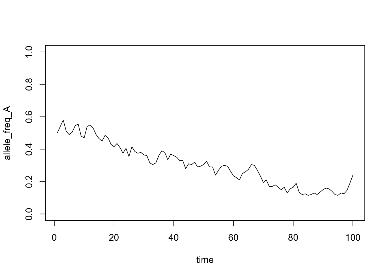
Figure 17.1: Simulation of allele frequency through time
Use the code to investigate the following questions:
- How does population size affect the variation through time in allele frequencies? Why do you see these patterns?
- How does the probability of fixation change with population size?
- When the population size is large (say 1000), is it still possible for alleles to become fixed?
- Are rare alleles (defined with allele frequency) more or less likely to be lost than common ones? What implications does this have for new alleles (mutations)?
Tip: make a new script and paste the code loop along with the plot command so that you can run both together easily.
17.6 Bottlenecks
Well done for making it this far. R programming is not for the faint hearted.
Next up, I want you to take the code, and modify the code within the loop to simulate a genetic bottleneck. A genetic bottleneck occurs when the population goes through a period of small population size.
This code means, “…if the generation time is between 30 and 50, make the population size 10, otherwise make the population size 1000”. In other words, the population goes through a bottleneck period of 20 generations. You could modify this line of code to change the characteristics of the bottleneck.
Figure 17.2 shows an example of what your plot of a genetic bottleneck simulation may look like. I have added some lines to show where the bottleneck starts/ends.
# Set number of generations
n_gen <- 100
# Set up an empty vector of length n_gen to contain results
allele_freq_A <- rep(NA, n_gen)
# Put in an initial value for frequency of A
allele_freq_A[1] <- 0.5
# Establish the initial gene pool and name it gene_pool_time_n
# This part looks complicated, but I am just condensing the code from above into 1 line.
gene_pool_time_n <- c(
rep("A", round(2 * allele_freq_A[1] * pop_size)),
rep("a", round(2 * (1 - allele_freq_A[1]) * pop_size))
)
for (i in 2:n_gen) {
if (i %in% 30:50) {
pop_size <- 15
} else {
pop_size <- 1000
}
gene_pool_time_n_plus_1 <- sample(gene_pool_time_n,
pop_size * 2,
replace = TRUE
)
gene_pool_table <- table(gene_pool_time_n_plus_1)
allele_freq_A[i] <- gene_pool_table[2] / sum(gene_pool_table)
# Replace the old gene pool with the new one.
gene_pool_time_n <- gene_pool_time_n_plus_1
}
plot(1:n_gen, allele_freq_A, type = "l",
     xlab = "time",
     ylim = c(0, 1))
abline(v = 30,col= "red", lty = 3)
abline(v = 50,col= "red", lty = 3)
text(40,0.95,"bottleneck", col = "red")
Figure 17.2: Simulation of a genetic bottleneck
Now use your new bottleneck code to answer the following questions:
- How does a genetic bottle neck influence the genetic composition of the population?
- How might a genetic bottleneck impact the probability of genetic fixation?
- Does the severity of the bottleneck (i.e. length and population size) matter?
17.7 Conclusions
You should now have a good idea of what a gene pool model is, the importance of population size, the concept of sampling from a population and genetic bottlenecks.
Let’s finish with some more general questions:
- What are the limitations of this simulation. What other real-world factors and complexities are not considered in this simplified model?
- Why is genetic diversity important to a population, for example in a conservation context?
- Can you think of real-life scenarios where understanding gene pool dynamics would be valuable, such as in conservation biology or medical genetics?
17.8 Takeaways
Genetic drift is stronger in small populations because sampling error is larger.
Bottlenecks and founder effects can rapidly reshape allele frequencies.
Even neutral processes can lead to fixation or loss over time.
Can you think of a way to simulate the genetics of a population that is steadily shrinking through time?