16 Hardy-Weinberg equilibrium
16.1 Background
Hardy-Weinberg equilibrium is a fundamental concept in population genetics for understanding the genetic dynamics of populations. Named after British mathematician G.H. Hardy and German physician Wilhelm Weinberg, this principle describes the stable genetic proportions in a population under specific conditions of no evolution.
In an idealized population, where mating is random, genetic mutations are absent, natural selection is not acting, and there is no gene flow or genetic drift, the frequencies of alleles and genotypes remain constant across generations.
The Hardy-Weinberg equilibrium provides a baseline against which real populations can be compared, allowing researchers to detect factors that may cause deviations from this equilibrium and, in turn, understand the forces driving evolution and genetic changes within populations.
In this practical we will learn more about HWE and practice solving some HWE-related problems.
The key formulae of the Hardy-Weinberg Equilibrium are:
Equation 1: \(p + q = 1\)
and
Equation 2: \(p^2 + 2pq + q^2 = 1\).
Let’s first consider where these equations come from. First, Equation 1.
In a diploid organism, each individual carries two alleles for a particular gene. Let’s consider a gene with two alleles, A and a. In a given population:
\(p\) is the frequency of the dominant allele (A) \(q\) is the frequency of the recessive allele (a)
The sum of the frequencies of these two alleles in the population must equal 1, as they are the only two possibilities for this gene, so \(p+q=1\).
Equation 1 serves as the foundational stepping stone for Equation 2. In Equation 1, we establish the sum of allele frequencies, \(p\) and \(q\), in the gene pool. This equation sets the stage for the more complex Equation 2, where we translate these allele frequencies into genotype frequencies for the population.
We can derive Equation 2 based on the gene pool and random mating. Let’s consider a mating event between two random alleles. The possible combinations of alleles are:
\(p \times p = p^2\) (AA) \(q \times q = q^2\) (aa) \(p \times q = pq\) (Aa) \(q \times p = pq\) (aA)
Notice that we have two \(pq\) terms (Aa and aA). The order of alleles doesn’t matter, so they are summed together: \(2pq\).
So, the total probability for all possible combinations is:
\(p^2 + 2pq + q^2\).
This must equal 1 (100% probability), which gives us Equation 2:
\(p^2 + 2pq + q^2 = 1\).
In these formulae, \(p\) is the allele frequency of the dominant allele and \(q\) is the frequency of the recessive allele. Thus, \(p^2\) is the frequency of the homozygous dominant genotype (e.g., AA), \(q^2\) is the frequency of the homozygous recessive genotype (e.g., aa) and \(2pq\) is the frequency of the heterozygous genotype (e.g., Aa). From these equations we can produce the following plot that shows the possible genotype frequencies at HWE for any given pair of allele frequencies. HWE can be reached for any genotype frequency (it is a common misconception that ratios between the three genotypes should be 1:2:1, or that allele frequencies should tend towards being 50% \(p\) and 50% \(q\)).
Given a small amount of information it is possible to figure out what the allele and genotype frequencies should be if the population is at HWE.
If the population is NOT at HWE, then it must be that one of the assumptions is violated.
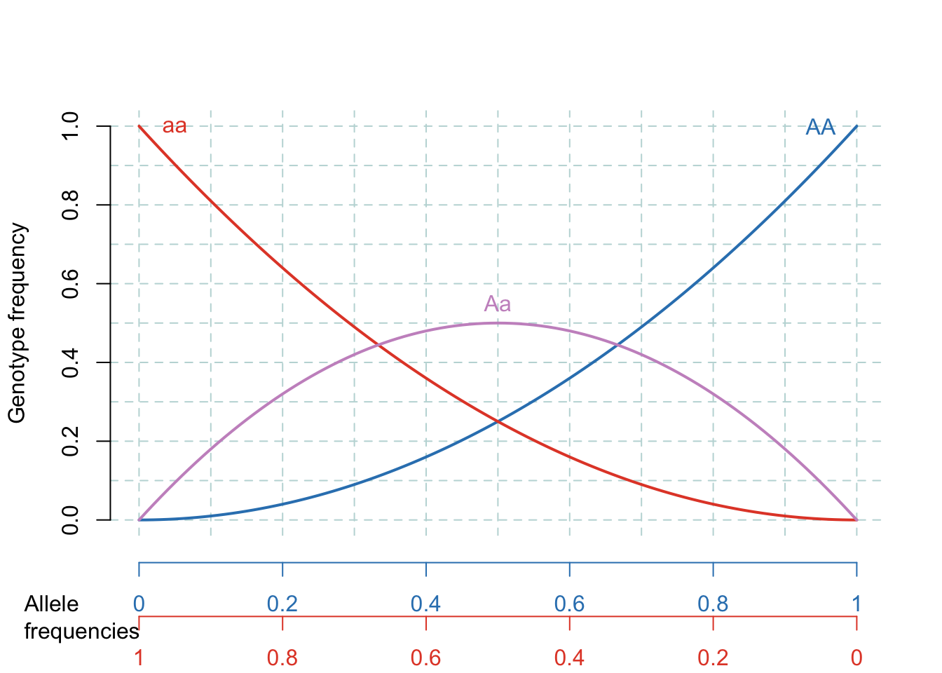
Figure 16.1: The Hardy-Weinberg Equilibrium. The lines represent the genotype frequencies at HWE, given particular allele frequencies.
16.2 Assumptions of Hardy-Weinberg Equilibrium
For a population to be in Hardy-Weinberg Equilibrium, certain assumptions must be met:
- Random mating: There is no preference in mate selection based on genotype.
- No mutations: The gene pool is stable with no new alleles being added.
- Large population size: To negate the effects of genetic drift.
- No gene flow: No new individuals enter or leave the population.
- No natural selection: All genotypes in the population have an equal chance of reproductive success.
Any deviation from these assumptions could result in a population that is not in Hardy-Weinberg Equilibrium.
Learning outcomes:
- Understanding the difference between alleles and genotypes.
- The ability to solve Hardy-Weinberg problems by understanding and applying the two key formulae of HW.
- Knowing the assumptions of HWE.
- Understanding what “being at Hardy-Weinberg Equilibrium” means in terms of evolutionary processes (which is related to the assumptions of HWE).
16.3 Worked example
16.4 Your task
Tackle the following problems, using the HWE theory outlined above …
16.4.1 Problem #1.
You have sampled a population in which you know that the percentage of the homozygous recessive genotype (aa) is 36%. Using that 36%, calculate the following:
- The frequency of the “aa” genotype.
- The frequency of the “a” allele.
- The frequency of the “A” allele.
- The frequencies of the genotypes “AA” and “Aa.”
- The frequencies of the two possible phenotypes if “A” is completely dominant over “a.”
16.4.2 Problem #2.
Sickle-cell anaemia is an interesting genetic disease. Normal homozygous individuals (SS) have normal blood cells that are easily infected with the malarial parasite. Thus, many of these individuals become very ill from the parasite and many die. Individuals homozygous for the sickle-cell trait (ss) have red blood cells that readily collapse when deoxygenated. Although malaria cannot grow in these red blood cells, individuals often die because of the genetic defect. However, individuals with the heterozygous condition (Ss) have some “sickling” of red blood cells (where the cells become C-shaped), but generally not enough to cause mortality. In addition, malaria cannot survive well within these “partially defective” red blood cells. Thus, heterozygotes tend to survive better than either of the homozygous conditions.
- If 9% of an African population is born with a severe form of sickle-cell anaemia (ss), what percentage of the population will be more resistant to malaria because they are heterozygous for the sickle-cell gene?
16.4.3 Problem #3.
There are 100 students in a class. Ninety-six did well in the course whereas four blew it totally and received a grade of F. In the highly unlikely event that these traits are genetic rather than environmental, if these traits involve dominant and recessive alleles, and if the four (4%) represent the frequency of the homozygous recessive condition, please calculate the following:
- The frequency of the recessive allele.
- The frequency of the dominant allele.
- The frequency of heterozygous individuals.
Note: This scenario is hypothetical and simplifies the complex factors that contribute to academic performance for the sake of this exercise. Academic performance is influenced by a myriad of factors, not solely genetics!
16.4.4 Problem #4.
Within a population of butterflies, the colour brown (B) is dominant over the colour white (b). And, 40% of all butterflies are white. Given this simple information calculate the following:
- The percentage of butterflies in the population that are heterozygous.
- The frequency of homozygous dominant individuals.