23 Discrete-time Lotka-Volterra Predator-Prey Model in R
23.1 Learning outcomes
Learning outcomes:
- Implement and explore a discrete-time predator-prey model in R.
- Understand how time steps introduce delays and affect stability.
- Compare discrete-time dynamics to continuous-time dynamics.
23.2 Key idea
With \(\Delta t = 1\), the phase plane typically shows expanding spirals, reflecting instability introduced by discrete time steps.
23.3 Introduction
The Lotka-Volterra model describes the interaction between predators and prey. This document demonstrates how to program the discrete-time version of the model in R, explore its features, and visualise the dynamics of predator and prey populations over time. The time step (\(\Delta t\)) can be adjusted to explore the impact of a time delay in the system. In ecological systems, time delays can represent biological processes such as the time it takes for predators to respond to changes in prey density, for prey populations to recover after predation. If \(\Delta t\) is set to 1, this model is equivalent to a year-by-year model (as we have fitted in Excel in class), where the impact of predators on prey has a 1 year lag. i.e. the growth of predators, depends on the availability of prey 1 year ago and the growth of prey depends on the amount of predators 1 year ago.
23.4 Step 1: Define the Model
The discrete-time equations are as follows:
Victim (prey) population growth:
\(V_{t+1} = V_t + \Delta t \cdot (R \cdot V_t - a \cdot C_t \cdot V_t)\)Consumer (predator) population growth:
\(C_{t+1} = C_t + \Delta t \cdot (a \cdot f \cdot V_t \cdot C_t - q \cdot C_t)\)
Note that, when \(\Delta t = 1\), the model is as follows:
Victim (prey) population growth:
\(V_{t+1} = V_t + R \cdot V_t - a \cdot C_t \cdot V_t\)Consumer (predator) population growth:
\(C_{t+1} = C_t + a \cdot f \cdot V_t \cdot C_t - q \cdot C_t\)
Compare these to Equations 1 and 2 in the Excel exercise PDF.
The function below implements these equations in R.
discrete_predator_prey_model <- function(time_steps, dt, initial_state, parameters) {
  # Initialise vectors to store populations
  V <- numeric(time_steps + 1)
  C <- numeric(time_steps + 1)
  time <- seq(0, time_steps * dt, by = dt)

  # Set initial populations
  V[1] <- initial_state["V"]
  C[1] <- initial_state["C"]

  # Extract parameters
  R <- parameters["R"]
  a <- parameters["a"]
  f <- parameters["f"]
  q <- parameters["q"]

  # Loop through time steps to calculate populations
  for (t in 1:time_steps) {
    V[t + 1] <- V[t] + dt * (R * V[t] - a * V[t] * C[t])
    C[t + 1] <- C[t] + dt * (a * f * V[t] * C[t] - q * C[t])
  }

  # Combine results into a data frame
  data.frame(time = time, V = V, C = C)
}
23.5 Step 2: Set Parameters and Initial Conditions
We set the parameters, initial conditions, and time step (\(\Delta t\)) for the model.
parameters <- c(R = 0.25,  # Victim (prey) growth rate
                a = 0.01,  # Attack rate
                f = 0.008, # Conversion efficiency
                q = 0.1)   # Consumer (predator) death rate

initial_state <- c(V = 1000,  # Initial victim population
                   C = 20)    # Initial consumer population

time_steps <- 200             # Number of time steps
dt <- 1 # Time step (dt), 1 = a standard discrete model23.7 Step 4: Visualise the Dynamics
23.7.1 Population Dynamics Over Time
The plot below shows the changes in consumer and victim populations over time.
# Plot victim population on the primary y-axis
plot(output_df$time, output_df$V, type = "l", col = "blue", lwd = 2,
     ylab = "Victim Population (V)", xlab = "Time", main = "Discrete Predator-Prey Dynamics")

# Add consumer population on a secondary y-axis
par(new = TRUE)
plot(output_df$time, output_df$C, type = "l", col = "red", lwd = 2,
     axes = FALSE, xlab = "", ylab = "")
axis(side = 4, col = "red", col.axis = "red")
mtext("Consumer Population (C)", side = 4, line = 3, col = "red")

# Add legend
legend("topright", legend = c("Victim (V)", "Consumer (C)"),
       col = c("blue", "red"), lwd = 2)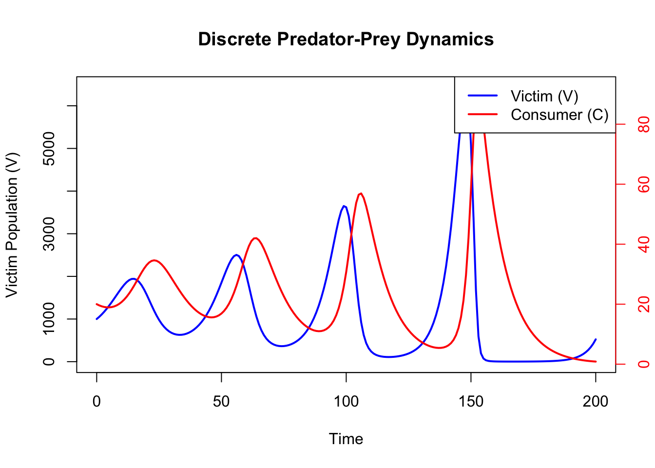
23.7.2 Phase Plot with ZNGIs
The phase plot shows the relationship between victim and consumer populations.
### Phase Plot with ZNGIs, Initial Point, and Arrow
plot(output_df$V,
     output_df$C,
     type = "l",
     col = "purple",
     lwd = 2,
     xlab = "Victim (V)", ylab = "Consumer (C)",
     main = "Discrete Predator-Prey Dynamics with ZNGIs")

# Add Victim ZNGI (V = q / (a * f))
abline(v = parameters["q"] / (parameters["a"] * parameters["f"]),
       col = "blue", lwd = 2, lty = 2)

# Add Consumer ZNGI (C = R / a)
abline(h = parameters["R"] / parameters["a"], col = "red", lwd = 2, lty = 2)

# Add point for initial population sizes
points(output_df$V[1], output_df$C[1], pch = 19, col = "black", cex = 1.5)

# Add an arrow to the end of the line
arrows(x0 = output_df$V[nrow(output_df) - 1],
       y0 = output_df$C[nrow(output_df) - 1],
       x1 = output_df$V[nrow(output_df)],
       y1 = output_df$C[nrow(output_df)],
       col = "purple", length = 0.1, lwd = 2)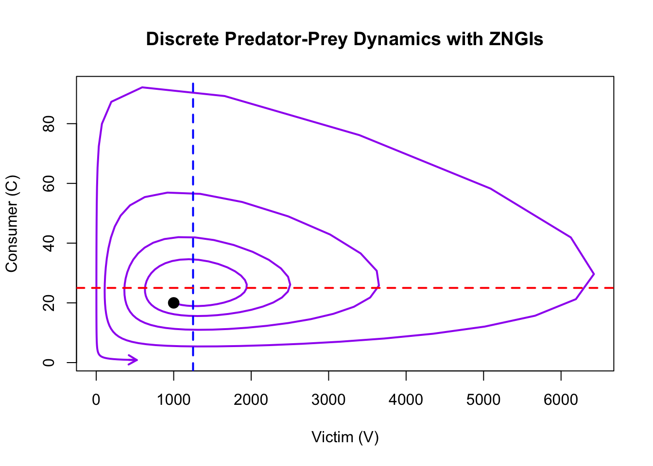
23.8 Conclusion
This document demonstrates how to implement and explore the discrete-time Lotka-Volterra predator-prey model. By adjusting the time step (\(\Delta t\)) and other parameters, you can investigate how predator-prey dynamics are influenced by ecological factors. You will see that a time lag imposed by the t parameter results in expanding spirals in the phase plot and eventual extinction of predator and prey. Contrast this with the perpetual oscillations you get with the continuous time model.