Compute 95% confidence intervals for derived estimates from a matrix population model

This function computes the 95% confidence interval for measures derived from a matrix population model using parametric bootstrapping. In this approach a sampling distribution of the matrix population model (MPM) is generated by taking a large number of random independent draws using the sampling distribution of each underlying transition rate. The approach rests on our assumption that survival-related processes are binomial, while fecundity is a Poisson process (see the function add_mpm_error() for details).

Usage

compute_ci(mat_U, mat_F, sample_size, FUN, ..., n_sim = 1000, dist.out = FALSE)

Arguments

mat_U: A matrix that describes the growth and survival process.
mat_F: A matrix that describes fecundity.
sample_size: either (1) a single matrix of sample sizes for each element of the MPM, (2) a list of two named matrices ("mat_F_ss", "mat_U_ss") containing sample sizes for the survival and fecundity submatrices of the MPM or (3) a single value applied to the whole matrix
FUN: A function to apply to each simulated matrix population model. This function must take, as input, a single matrix population model (i.e., the A matrix). For functions that require only the U matrix, use compute_ci_U.
...: Additional arguments to be passed to FUN.
n_sim: An integer indicating the number of simulations to run. Default is 1000.
dist.out: Logical. If TRUE, returns a list with both the quantiles and the simulated estimates. Default is FALSE.

Value

If dist.out is FALSE, a numeric vector of the 2.5th and 97.5th quantiles of the estimated measures. If dist.out = TRUE, a list with two elements: quantiles and estimates. quantiles is a numeric vector of the 2.5th and 97.5th quantiles of the estimated measures, and estimates is a numeric vector of the estimated measures.

Details

The inputs are the U matrix, which describes the survival-related processes, and the F matrix which describes fecundity. The underlying assumption is that the U matrix is the average of a binomial process while the F matrix is the average of a Poisson process . The confidence interval will depend largely on the sample size used.

References

Chapter 12 in Caswell, H. (2001). Matrix Population Models. Sinauer Associates Incorporated.

Author

Owen Jones jones@biology.sdu.dk

Examples

set.seed(42) # set seed for repeatability

# Data for use in example
matU <- matrix(c(
  0.1, 0.0,
  0.2, 0.4
), byrow = TRUE, nrow = 2)

matF <- matrix(c(
  0.0, 5.0,
  0.0, 0.0
), byrow = TRUE, nrow = 2)

set.seed(42)

# Example of use to calculate 95% CI of lambda
compute_ci(
  mat_U = matU, mat_F = matF, sample_size = 10, FUN =
    popbio::lambda
)
#>     2.5%    97.5% 
#> 0.300000 1.824895 

# Example of use to calculate 95% CI of generation time
compute_ci(
  mat_U = matU, mat_F = matF, sample_size = 40, FUN =
    popbio::generation.time
)
#>     2.5%    97.5% 
#> 2.386966 3.072293 

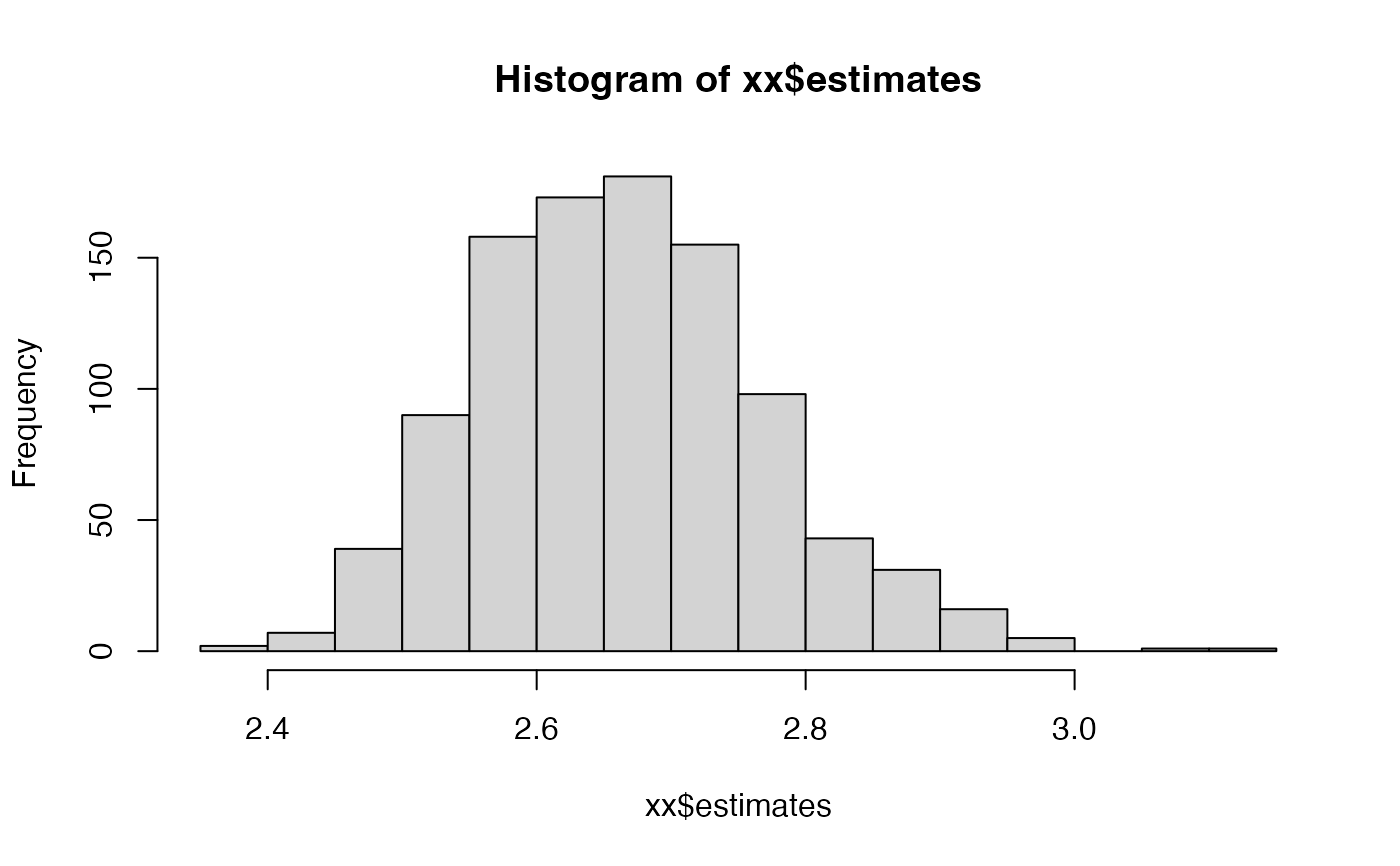
# Example of use to calculate 95% CI of generation time and show the
# distribution of those bootstrapped estimates
xx <- compute_ci(
  mat_U = matU, mat_F = matF, sample_size = 100, FUN =
    popbio::generation.time, dist.out = TRUE
)
summary(xx$quantiles)
#>    Min. 1st Qu.  Median    Mean 3rd Qu.    Max. 
#>   2.476   2.581   2.686   2.686   2.791   2.896 
hist(xx$estimates)